Two-Phase Flow Regimes in Gas-Liquid Pipes: A Complete Engineering Guide

In any pipeline system where gas and liquid coexist, the way the two phases distribute themselves inside the pipe—the flow regime—has a direct and significant impact on pressure drop, liquid holdup, vibration, and overall system integrity. Unlike single-phase flow, where the hydraulic behavior can be described with a single set of equations, two-phase gas-liquid flow presents a far more complex picture: the mixture can arrange itself into several distinct patterns depending on operating conditions, fluid properties, and pipe geometry.

Identifying the correct flow regime is not merely an academic exercise—it is an engineering prerequisite. Different regimes call for different pressure-drop correlations, different approaches to liquid holdup calculation, and different mechanical design considerations. Getting the flow regime wrong can lead to oversized pipes, or in the worst case, undetected slug flow that imposes damaging pulsating loads on the piping structure.

This article provides a comprehensive overview of two-phase flow regimes in gas-liquid pipes, covering both horizontal and vertical orientations, the flow regime maps engineers use to identify them, the effect of pipe inclination, and how FluidFlow’s two-phase flow simulation software automates and accelerates this analysis.

What Determines the Flow Regime?

When gas and liquid flow together inside a pipe, the mixture can exhibit many different flow patterns. The prevailing regime at any given point is governed by five key factors:

• Fluid physical properties — density (ρ), dynamic viscosity (μ), and surface tension (γ)
• Pipe diameter
• Gas volumetric flow rate (Q_G)
• Liquid volumetric flow rate (Q_L)
• Pipe orientation — horizontal, vertical, or inclined

Because so many variables interact, no single universal equation can predict the flow regime analytically. Instead, engineers rely on flow regime maps—graphical tools that plot the observed regime as a function of two key parameters, most commonly the superficial velocities of the gas and liquid phases. The superficial velocity of a phase is defined as the velocity that the phase would have if it occupied the entire cross-sectional area of the pipe alone.

Two-Phase Flow Regimes in Horizontal Pipes

Horizontal pipelines and near-horizontal configurations up to approximately 30 degrees of inclination exhibit six primary flow regimes, each with distinct hydraulic characteristics.

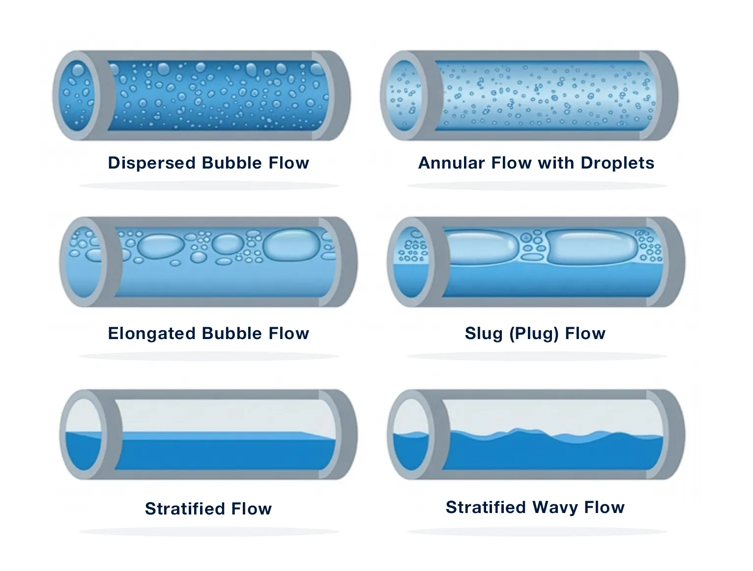
Figure 1: Common Flow Regimes in Two-Phase Flow in Horizontal Pipelines

1. Stratified Flow

Stratified flow occurs at low superficial velocities of both the gas and liquid phases. Gravity separates the two phases: the liquid settles along the bottom of the pipe, and the gas occupies the upper portion, with a distinct, relatively smooth interface between them. Because the interface is calm, this regime produces the most predictable and stable pressure gradients of all horizontal flow patterns. It is strictly a low-velocity phenomenon and is found in the lower-left region of the Mandhane-Gregory-Aziz flow regime map, corresponding to liquid superficial velocities below approximately 0.3 m/s and gas superficial velocities between 0.6 and 3.0 m/s.

2. Stratified Wavy Flow

As the superficial gas velocity exceeds the range that supports smooth stratified flow, the faster-moving gas disturbs the liquid surface, creating a wavy interface. This is stratified wavy flow. The wave structure increases turbulence in the liquid phase and causes a degree of gas entrainment into the liquid. The additional turbulence and the disturbed interface alter the pressure gradient compared to smooth stratified flow.

3. Elongated Bubble Flow

If the superficial liquid velocity is increased from stratified conditions, the flow transitions to elongated bubble flow—an intermittent regime. Collisions between individual gas bubbles occur more frequently as the gas flow rate increases, causing them to coalesce into elongated plugs that can extend many hundreds of pipe diameters in length. The elongated bubbles are characterized by a smooth interface with a distinct nose and tail shape. Between consecutive bubbles, liquid slug regions form in which there is very little gas entrainment. The velocity of the liquid within the slug region is essentially equal to the velocity of the gas in the elongated bubble ahead of it.

4. Slug (Plug) Flow

With a further increase in superficial gas velocity, elongated bubble flow transitions into slug flow—the most commonly encountered and most problematic regime in industrial piping. In slug flow, large, high-velocity gas slugs alternate periodically with liquid plugs along the pipe. The leading edge of each liquid slug is highly turbulent, with strong gas entrainment evident. A residual liquid film remains on the pipe walls after each slug passes.

Engineering Note: Slug flow is common across a wide range of gas and liquid superficial velocities that coincide with those found in many commercial pipelines. The pulsating, high-energy slugs generate significant mechanical stress on the piping system. If slug flow is anticipated, the piping stress team must be notified so that adequate pipe supports can be specified to prevent fatigue and excessive vibration.

5. Dispersed Bubble Flow

At high liquid superficial velocities, typically between 1.5 and 5 m/s, combined with moderate gas velocities, between 0.3 and 3.0 m/s, the dominant liquid phase generates high levels of turbulence that break the gas into very small, uniformly distributed bubbles. This is dispersed bubble flow: a continuous, homogeneous, frothy flow where the gas bubbles travel at approximately the same velocity as the liquid. A key feature of this regime is the potential for a ‘no-slip’ condition, where the phase velocity difference is negligible, which simplifies certain pressure-drop calculations significantly.

6. Annular Mist Flow (Annular Flow with Droplets)

At very high superficial gas velocities, the gas core becomes energetic enough to sustain a continuous liquid film along the pipe wall—forming the ‘annulus’—while entrained liquid droplets are carried in the high-velocity gas core at the center. This is annular mist flow. The film is thinner at the top of the pipe than at the bottom due to gravity, and the interface is rough and highly turbulent owing to the intense gas-liquid shear. As gas velocity increases further, almost all the liquid is entrained as fine droplets in the gas stream—a condition sometimes called spray, dispersed, or mist flow. Pressure gradients in this regime tend to be very high.

Two-Phase Flow Regimes in Vertical Pipes

Vertical and near-vertical piping with inclinations between 75 and 90 degrees supports a different set of flow regimes. The most immediately notable difference from horizontal flow is that stratified flow does not occur in vertical pipes. Because gravity acts uniformly along the pipe axis in vertical flow, it cannot drive the gravity-based phase separation that creates the characteristic liquid-bottom, gas-top arrangement of stratified flow. The regimes present in vertical systems are:

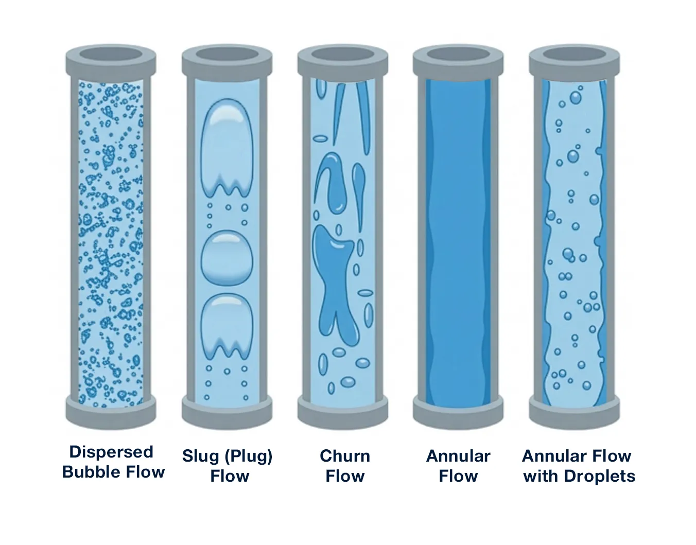
Figure 2: Common Flow Regimes in Two-Phase Flow in Vertical Pipelines

• Dispersed Bubble Flow — small gas bubbles uniformly distributed in a continuous upward liquid stream at high liquid velocity.
• Slug (Plug) Flow — large, bullet-shaped Taylor bubbles alternate with liquid slugs. In vertical piping, this regime is commonly associated with hilly terrain systems, where low points accumulate liquid and promote slug formation.
• Churn (Froth) Flow — a highly turbulent, disordered regime at elevated gas velocities, where large irregular gas slugs rise chaotically through the pipe center, carrying entrained liquid droplets. There is no stable gas-liquid interface. Churn flow imposes strong pressure fluctuations and vibration forces and is generally undesirable in design.
• Annular Flow — at high gas velocities, the chaotic churn pattern reorganizes into a stable annular configuration, with a continuous gas core carrying entrained droplets and a thin liquid film coating the pipe wall. This is the terminal regime as gas velocity increases regardless of pipe orientation.

The fundamental flow mechanism and pressure-drop behavior differ for each of these patterns, making it critical from a design standpoint to predict which regime will prevail for a given set of operating conditions in a vertical segment.

Effect of Pipe Inclination on Flow Regimes

One of the most striking and practically important observations in two-phase flow is how sensitive the flow regime is to pipe inclination—even a minor change in angle can produce a dramatically different flow pattern. Consider a horizontal pipe operating under stratified flow conditions. Tilting that pipe upward by just a few degrees immediately breaks down the stable stratified pattern and induces a transition to elongated bubble flow. This occurs because even a slight upward inclination introduces a gravitational component along the pipe axis that destabilizes the liquid-gas interface.

Furthermore, in inclined pipes, a reverse liquid flow develops in the liquid film between consecutive slugs—meaning the liquid is locally flowing backward against the primary direction of flow. This reverse-flow phenomenon significantly influences liquid holdup, pressure drop, and system stability.

This confirms a critical design principle: flow regime is not determined solely by fluid velocities and physical properties. Pipe orientation is an equally important variable, and even small deviations from horizontal—whether upward or downward—must be carefully accounted for when selecting a two-phase flow correlation and predicting system behavior in cross-country or hilly-terrain pipelines.

Flow Regime Maps

Several flow regime maps have been developed over the decades to help engineers identify the prevailing regime. Each has its own coordinate system, data basis, and range of applicability.

Baker Chart (1958)

The Baker Chart, published in the Oil and Gas Journal in 1958, was among the first widely adopted flow pattern maps for horizontal two-phase flow. It identifies six regimes—Wave, Stratified, Slug, Plug, Annular, and Dispersed—using two calculated parameters (Bx and By) derived from phase mass flow rates, densities, viscosity, and surface tension. While historically significant, the Baker Chart was developed primarily for large pipe diameters and fluid properties approximating air and water at atmospheric pressure. For systems with significantly different properties—high-pressure steam, hydrocarbons, or other process fluids—this map may not produce reliable results and should be used with caution.

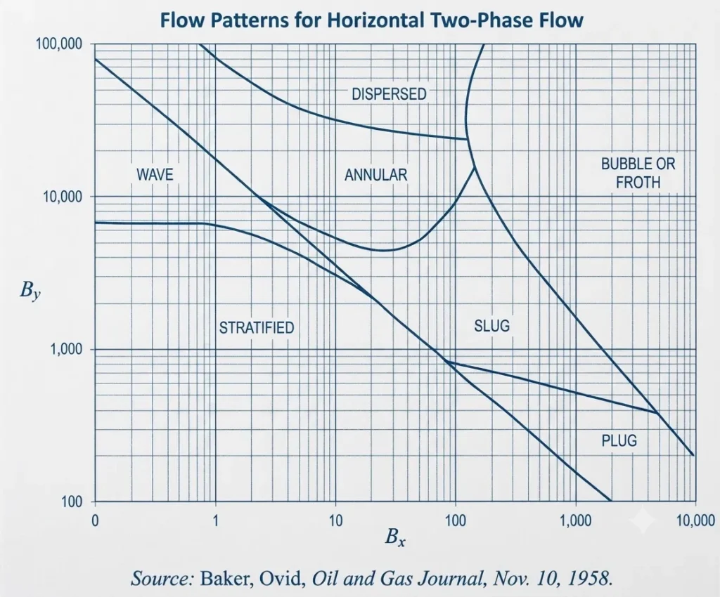
Figure 3: Baker Plot for Horizontal Two-Phase Flow. Adapted from Baker, Ovid, Oil and Gas Journal, Nov. 10, 1958.

Mandhane, Gregory, and Aziz Map

Developed through experimental research at a Canadian university, the Mandhane-Gregory-Aziz map plots superficial gas velocity on the horizontal axis against superficial liquid velocity on the vertical axis. This coordinate system is intuitive and is widely used. The map clearly delineates the boundaries between stratified, stratified wavy, elongated bubble, slug, dispersed bubble, and annular mist regimes, making it a practical reference tool for horizontal flow analysis.

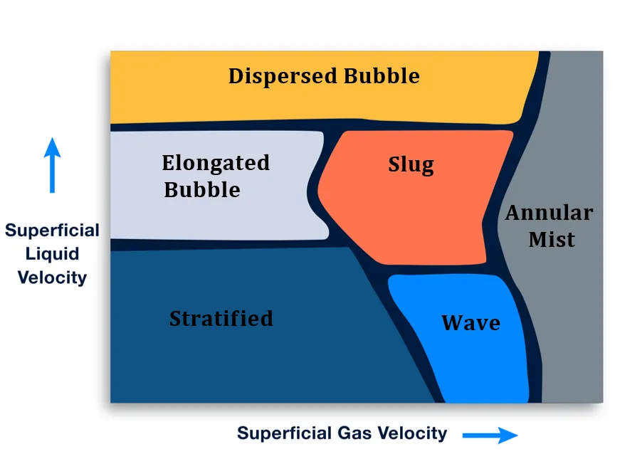
Figure 4: Flow pattern map for horizontal gas-liquid flow.  Adapted from Mandhane, Gregory, and Aziz (1974) 

Beggs and Brill Map

The Beggs and Brill correlation identifies the flow pattern using a horizontal flow-pattern map built on two parameters: the Froude number of the mixture and the input liquid content (no-slip liquid holdup). Observed flow patterns are grouped into four categories: segregated (stratified, wavy, and annular flow), intermittent (plug and slug flow), distributed (bubble and mist flow), and transition. The correlation is applicable to inclined pipes and is one of the eight industry-standard correlations available in FluidFlow for calculating frictional pressure loss in two-phase systems.

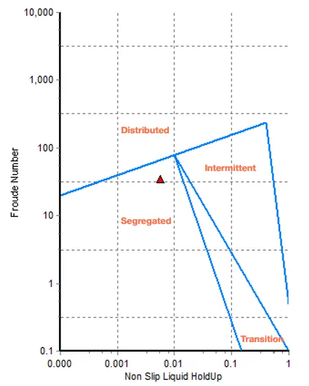
Figure 5: Beggs and Brill flow Pattern map in FluidFlow. 

Petalas and Aziz Mechanistic Model (FluidFlow Primary Approach)

For most two-phase flow calculations, FluidFlow uses the Petalas and Aziz mechanistic model (2000) with flow maps plotted as superficial gas velocity (x-axis) against superficial liquid velocity (y-axis). Unlike empirical correlations developed for specific data sets, the Petalas and Aziz model applies first principles to the possible flow patterns at different pipe inclinations. It is therefore applicable to any pipe inclination and a wide range of fluid properties. The model was refined from an earlier 1996 study, validated against a database of over 20,000 laboratory measurements and approximately 1,800 well measurements.

The method works by assuming a flow pattern, evaluating whether that pattern is stable under the given conditions, and—if stable—proceeding to calculate liquid holdup and the friction factor for pressure loss calculation. If no stable pattern is found, the flow is designated as froth, representing a transitional state between regimes.

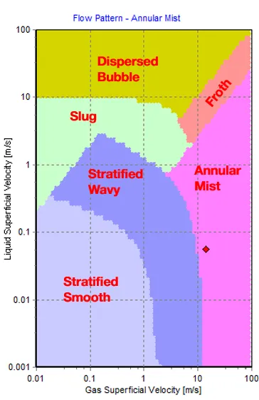
Figure 6: Petalas and Aziz flow Pattern map in FluidFlow. 

Modeling Two-Phase Flow Regimes with FluidFlow

Accurately predicting two-phase flow regimes in a real pipeline network—with multiple pipe segments at varying inclinations, changing pressures, and evolving phase fractions—is a task that quickly exceeds what can be done manually. FluidFlow’s two-phase flow simulation module is designed to automate and accelerate exactly this kind of analysis. Here is how its key features support two-phase flow regime engineering:

Automatic Flow Regime Mapping

FluidFlow automatically generates a flow regime map for every pipe segment in the network, identifying whether each segment operates in slug, annular, bubbly, stratified, or another regime. This per-segment mapping allows engineers to pinpoint locations of potential vibration risk (slug flow), erosion risk (annular mist), or operational concern (churn flow in vertical sections) without manual calculation.

Comprehensive Correlation Library

FluidFlow provides eight industry-standard correlations for calculating frictional pressure loss in two-phase flow, including Friedel, Chisholm-Baroczy, Lockhart-Martinelli, Drift Flux, Beggs and Brill, Muller-Steinhagen-Heck, and Homogeneous Equilibrium Model. The software can automatically select the optimal correlation based on fluid properties and flow conditions, eliminating the guesswork involved in manual correlation selection—a significant time saving in complex or multi-fluid systems.

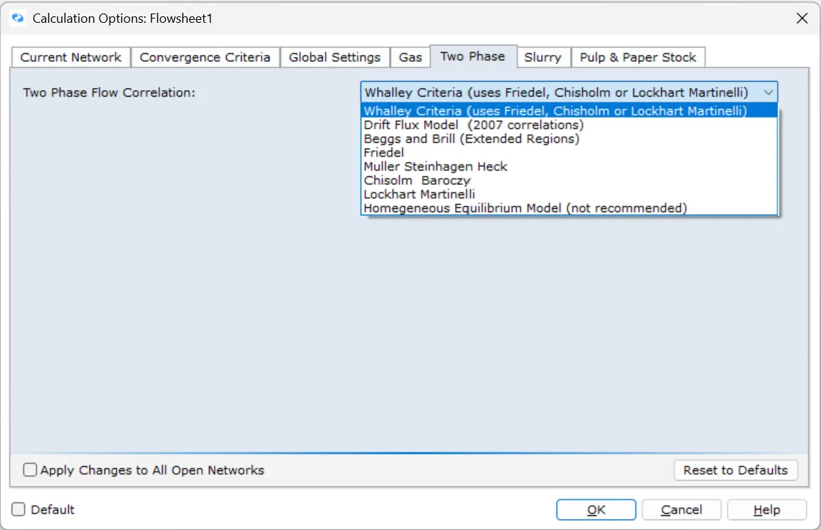
Figure 7: Two-Phase Flow Pressure Drop Correlations in FluidFlow. 

Phase Change and Flash Calculations

As pressure drops along a pipeline, liquids can flash to vapor and vapors can condense, changing the local vapor quality and, consequently, the local flow regime. FluidFlow performs rigorous flash calculations to determine vapor quality changes resulting from pressure drops or heat transfer, ensuring that the flow regime prediction remains accurate along the full length of the pipe. This capability is particularly valuable for steam condensate lines, geothermal steam gathering networks, and chemical plant overhead piping.

Multi-Fluid Mixing and Phase Tracking

When different fluid streams converge in a network, FluidFlow handles the transition from single-phase to multi-phase automatically, tracking vapor quality along every flow path. This continuous phase tracking means the software always knows the local thermodynamic and flow state in each pipe segment, an essential requirement for reliable flow regime identification and pressure-loss calculation.

Marching-Solution Algorithm

FluidFlow uses a marching-solution approach to solve two-phase flow networks: the pipe is divided into small segments, and the flow equations are solved sequentially from inlet to outlet, updating fluid properties, vapor quality, holdup, and flow regime at each step. This approach captures the spatial variation of two-phase flow behavior along the pipe length—including regime transitions—with a level of accuracy that a single-segment calculation cannot achieve.

Trusted by over 1,000 engineering companies worldwide—across power generation, chemicals, geothermal, and oil and gas—FluidFlow enables engineers to design two-phase systems up to 75% faster. A 14-day free trial is available at fluidflowinfo.com.

Frequently Asked Questions (FAQ)

What is a two-phase flow regime?

A two-phase flow regime—also called a flow pattern—describes the spatial arrangement of the gas and liquid phases inside a pipe. Common examples are stratified flow (liquid at the bottom, gas at the top), slug flow (alternating liquid slugs and gas plugs), and annular flow (gas core with a liquid wall film). The regime determines how the two phases interact and directly governs the pressure drop and liquid holdup in the pipe.

Why does the flow regime matter for engineering design?

Different regimes have fundamentally different pressure-drop behavior, holdup characteristics, and mechanical implications. Slug flow, for example, generates periodic high-pressure pulses that can cause pipe vibration and fatigue. Annular mist flow produces high pressure gradients and may lead to erosion in high-velocity conditions. Selecting the wrong correlation—one that assumes a different regime than actually exists—can produce pressure-drop errors large enough to invalidate an entire system design.

How does pipe orientation affect the flow regime?

Pipe orientation is one of the five key variables that govern the flow regime. In horizontal pipes, gravity drives phase separation laterally, producing stratified and wavy flows. In vertical pipes, gravity acts along the pipe axis and eliminates stratified flow entirely, instead producing slug, churn, and annular patterns. Even a small change in inclination—a few degrees up or down—can trigger a regime transition.

What is the Petalas and Aziz model, and why does FluidFlow use it?

The Petalas and Aziz mechanistic model (2000) applies first principles rather than empirical curve-fitting to predict two-phase flow patterns and calculate pressure loss. Because it is not tied to a specific data set or fluid type, it is applicable to any pipe inclination and a wide range of fluid properties—making it the most versatile general-purpose two-phase flow model available. FluidFlow uses this model as its primary approach for flow regime mapping and pressure-drop calculation.

Can FluidFlow handle flow regime changes along a pipeline?

Yes. FluidFlow uses a marching-solution algorithm that divides each pipe into small segments and solves the flow equations sequentially, updating fluid properties, vapor quality, liquid holdup, and flow regime at each step. This means that if a pipe transitions from slug flow near the inlet to annular flow further downstream—due to expanding gas as pressure drops—FluidFlow will capture that transition and apply the appropriate correlation for each section of the pipe.

Which industries benefit most from two-phase flow regime analysis?

Any industry handling simultaneous gas-liquid flow benefits. Common applications include steam condensate lines and boiler blowdown in power generation; overhead condenser lines, reflux drum outlets, and flare headers in chemicals and petrochemicals; steam gathering networks in geothermal energy; and production flowlines in oil and gas. FluidFlow supports all of these applications through its integrated two-phase flow module.

How do I get started with two-phase flow simulation in FluidFlow?

FluidFlow offers a 14-day free trial with full access to all simulation modules, including the two-phase flow module. The trial includes pre-built sample projects so you can start working with real two-phase flow problems immediately. Visit fluidflowinfo.com to download the trial—no credit card required.

Key Takeaways

• Flow regime identification is a prerequisite for any accurate two-phase flow calculation—pressure drop, liquid holdup, and mechanical design all depend on it.
• Horizontal pipes support up to six regimes: stratified, stratified wavy, elongated bubble, slug/plug, dispersed bubble, and annular mist. Vertical pipes replace stratified flow with churn flow.
• Slug flow is the most problematic regime in commercial piping systems, generating high-energy pulsations that can cause fatigue failure if pipe supports are not designed for it.
• Even a small change in pipe inclination can trigger a regime transition—stratified flow in a horizontal pipe can shift immediately to elongated bubble flow with just a few degrees of upward tilt.
• Flow regime maps—Baker Chart, Mandhane-Gregory-Aziz, Beggs and Brill, and Petalas and Aziz—each have different coordinate systems and ranges of applicability; the Petalas and Aziz mechanistic model offers the broadest applicability across inclinations and fluid properties.
• FluidFlow automatically identifies flow regimes, selects correlations, performs flash calculations, and tracks phase changes along every pipe segment.