Five Pitfalls That Distort Pipe Pressure Drop Calculations

🕑 9 min read

Piping and process engineers frequently face hydraulic discrepancies during commissioning, pump performance testing, or operational debottlenecking. A line sized on a quick design-phase spreadsheet often exhibits higher pressure loss or starved delivery points once installed in the plant. In many design workflows, engineers leave the main hydraulic model and rely on manual spreadsheets to reconcile pipe sizes, fitting allowances, surface roughness, and sizing criteria. When these isolated calculation shortcuts miss real hydraulic phenomena, downstream equipment selection and operating margins suffer. This article examines the five primary analytical pitfalls that distort pipe pressure drop calculations and establishes how to model line hydraulics accurately.

The Governing Principles of Pipe Pressure Drop

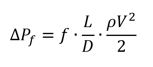
In single-phase fluid systems, the total pressure change across a conduit represents a mechanical energy balance between friction dissipation, potential energy from elevation changes, and kinetic energy from velocity variations. Frictional pressure drop in Newtonian fluids is governed by the Darcy-Weisbach equation:

Expressing fluid velocity in terms of volumetric flow rate $(V=4Q/(πD 2 ))$ reveals the extreme sensitivity of pressure drop to internal conduit diameter:

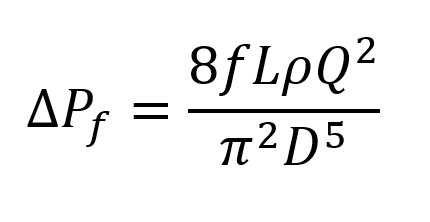
Because frictional resistance scales inversely with the fifth power of the internal pipe diameter (D⁵), a minor reduction in internal flow area creates a disproportionate increase in hydraulic head loss. Furthermore, the Darcy friction factor ( f ) depends on the flow regime characterized by the Reynolds number $Re=ρVD/μ$ and the relative surface roughness $(ε/D)$ . For laminar flow $(Re<2100)$ , viscous forces govern, and the friction factor follows Hagen-Poiseuille $(f=64/Re)$ , independent of wall roughness. In fully turbulent flow $(Re≥3100)$ , inertial forces dominate, requiring implicit solution of the Colebrook-White relationship where microscopic surface irregularities directly influence the energy dissipation rate.

Pressure Component	Governing Mechanism	Key Sensitivity Factors
Frictional Loss	Viscous shear and turbulent dissipation along pipe wall	Internal diameter (D5), absolute roughness (ε), Reynolds number (Re)
Elevation Differential	Static potential energy change (ρgΔz)	Fluid density (ρ), vertical elevation change (Δz)
Velocity Differential	Kinetic energy change $(Δ[ρV 2 /2])$	Cross-sectional area transitions, fluid density changes

Where Traditional Pipe Pressure Drop Calculations Break Down

Manual calculations, simplified rule-of-thumb tables, and standalone spreadsheets are standard tools across engineering offices. While they provide quick first-pass approximations, their underlying simplifications break down under common industrial operating conditions.

1. Conflating Nominal Pipe Size with Actual Internal Diameter

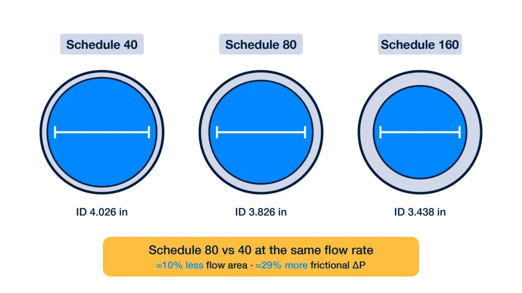
A widespread sizing error is using nominal pipe size (NPS or DN) instead of the actual internal diameter determined by the pipe wall schedule. A 4-inch (DN 100) pipe has an outside diameter of 4.500 inches (114.3 mm), but its internal diameter varies significantly across wall schedules. A standard Schedule 40 pipe has an inside diameter of 4.026 inches (102.3 mm), whereas an extra-strong Schedule 80 pipe has an inside diameter of 3.826 inches (97.2 mm), and Schedule 160 drops to 3.438 inches (87.3 mm).

Because frictional loss scales with 1/D5, substituting Schedule 80 for Schedule 40 in a 4-inch line reduces the flow area by approximately 10% and increases the frictional pipe pressure drop by nearly 29% at the same flow rate. Specifying high-pressure schedules or heavy corrosion allowances without updating hydraulic calculations leads directly to undersized lines and deficient terminal delivery pressures.

2. Assuming Constant Viscosity Across Temperature Variations

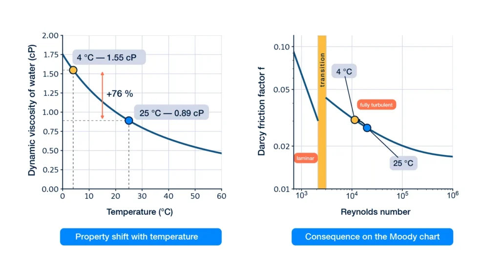
Many sizing spreadsheets treat fluid density and dynamic viscosity as static values evaluated at nominal ambient conditions. However, liquid viscosity is highly sensitive to temperature changes. For instance, water’s dynamic viscosity increases by roughly 78% as temperature drops from 25°C (0.89 cP) to 4°C (1.57 cP), while heavy hydrocarbons, glycols, and heat transfer fluids exhibit even steeper viscosity curves.

When an uninsulated outdoor line experiences winter ambient conditions, the resulting rise in viscosity lowers the Reynolds number. This shift can push a previously turbulent flow into the transition or laminar regime, driving up the friction factor and total pipe pressure drop. Assuming isothermal flow across lines with unmodeled heat loss produces overly optimistic pressure loss predictions.

3. Misapplying Empirical Formulas Outside Their Calibration Bounds

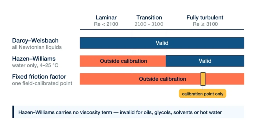
Engineers frequently apply the Hazen-Williams equation to industrial piping because it avoids the iterative calculation required by the Colebrook-White equation. Hazen-Williams relies on a dimensionless roughness constant (C-factor), typically set to 120–150 for commercial steel. However, the Hazen-Williams formula is an empirical correlation calibrated strictly for water at ambient temperatures (4°C to 25°C) in turbulent regimes.

Applying Hazen-Williams to oils, glycols, chemical solvents, or high-temperature water generates severe calculation errors because the formula contains no term for fluid viscosity. Furthermore, it cannot represent laminar flow or the Reynolds-number dependence of aged pipe roughness.

Friction Correlation	Applicable Fluid Range	Flow Regime Scope	Primary Limitation
Darcy-Weisbach (Moody)	All Newtonian liquids (water, oils, chemicals, solvents)	Laminar, transition, and fully turbulent	Requires iterative solution of Colebrook-White for turbulent flow
Hazen-Williams	Water only (4°C to 25°C)	Fully turbulent flow only	Ignores viscosity and temperature; invalid for non-water liquids
Shell-MIT	Heated, high-viscosity crude oils	Viscous (Re∗<0.135) and turbulent (Re∗≥0.4)	Treats pipe as hydraulically smooth; contains no roughness term
Fixed Friction Factor	Calibration against verified field data only	Fixed point conditions	Removes physical response to flow rate, viscosity, and roughness changes

4. Oversimplifying Fitting and Junction Resistances

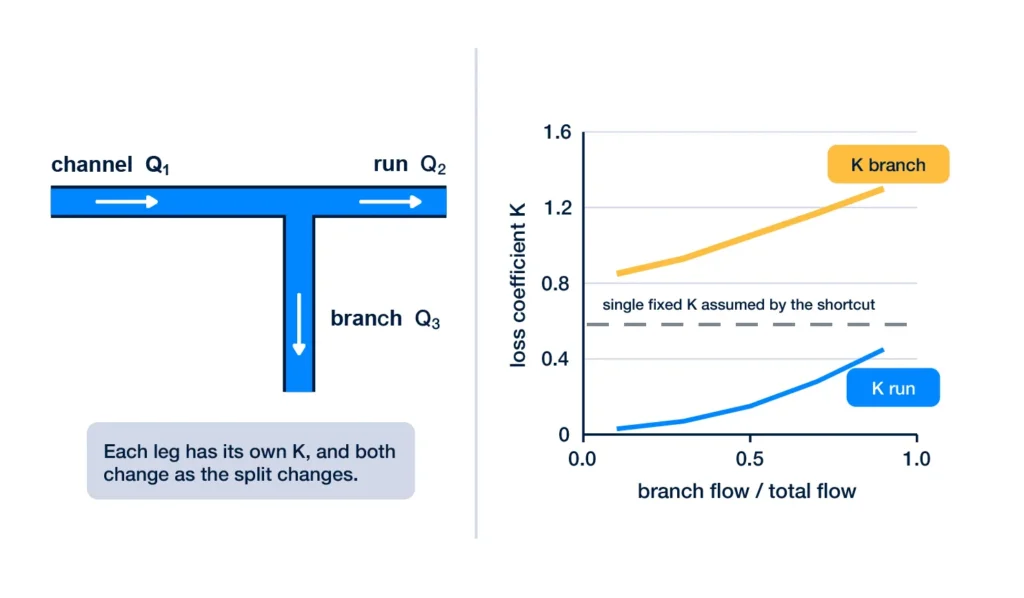
Standard engineering shortcuts often estimate minor losses by applying a flat percentage adder (such as adding 15% to total pipe length) or using fixed equivalent length ratios (L/D). These approximations misrepresent actual fitting behavior because minor loss coefficients (K) vary with fitting geometry, diameter reductions, and flow splits.

In branched distribution headers, treating a tee as a fixed resistance ignores the fundamental hydraulic difference between through-run flow and 90-degree branch extraction. Junction losses depend directly on the ratio of branch velocity to channel velocity. Misidentifying the branch leg or applying a generic single-fitting loss skews the pressure profile across the entire manifold.

5. Isolating Pipe Runs from Network Boundary Coupling

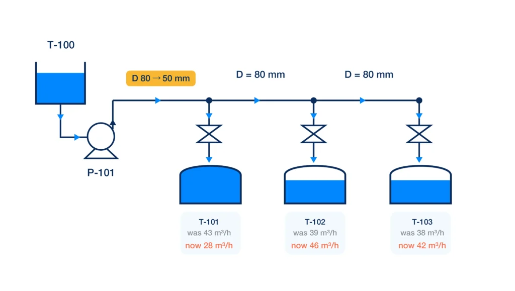
A single pipe run cannot be analyzed in isolation when it connects to parallel headers or shared manifolds. Hydraulic network solvers treat pressure and flow as simultaneously coupled variables, enforcing mass continuity at every junction and energy conservation around every loop.

When an engineer sizes an isolated line using a manual spreadsheet, they must assume fixed endpoint pressures. In an operating plant, changing the diameter or resistance of one branch redistributes flow across all adjacent branches sharing the common header. An isolated calculation cannot calculate this interactive flow redistribution.

Rigorous hydraulic software resolves the iterative complexity of network calculations while maintaining strict adherence to fluid mechanics principles. FluidFlow provides a dedicated environment to evaluate single lines and complex networks under verified Newtonian fluid correlations.

What FluidFlow Contributes to Pressure Drop Analysis

Rigorous Friction and Property Integration

When modeling liquid piping, FluidFlow utilizes Darcy-Weisbach as its core foundation, solving the Colebrook-White equation across turbulent regimes and Hagen-Poiseuille in laminar flow. The software accesses a physical property database of over 1,200 fluids to track density and viscosity changes along each pipe segment based on local operating temperatures.

For specialized services, FluidFlow provides alternative friction models, including Hazen-Williams for firewater compliance and Shell-MIT for heated crude oil transfer. Engineers can also activate pipe scaling to account for effective diameter reductions caused by mineral deposits or wax buildup over operating lifecycles.

Detailed Component and Junction Resistance Modeling

Instead of relying on crude equivalent-length approximations, FluidFlow evaluates discrete fittings and branched junctions using established loss correlations:

• Idelchik: Default correlation for tees, wyes, and complex fittings, calculating separate loss coefficients for run and branch streams while accounting for kinetic energy changes and area ratios.
• Miller: Rigorous junction modeling for converging and diverging flows with unequal connection sizes.
• Crane TP-410: Standard minor loss evaluations for turbulent fitting flows.
• SAE: Specialized resistance relationships for gas and utility networks.

FluidFlow requires explicit identification of branch and channel legs on directional components, allowing the solver to compute dynamic resistance as flow splits vary.

Automated Pipe Sizing Capabilities

To accelerate iterative line sizing across extensive networks, FluidFlow includes an automated Pipe Autosize utility. The software evaluates user-defined constraints and calculates the exact internal diameter required to satisfy the selected criterion:

Sizing Model	Underlying Basis	Typical Engineering Application
By Velocity	User-specified maximum target velocity	General liquid lines (e.g., maintaining liquid flow ≤2.0 m/s)
By Pressure Gradient	User-specified maximum allowable ΔP/L	Long transfer pipelines, pump suction lines, utility distribution headers
Economic Velocity	Generaux equation balancing capital and pumping energy costs	Continuous operating lines where lifecycle power consumption governs

Upon calculation, FluidFlow reports the exact theoretical diameter required. The engineer then selects the closest standard commercial pipe size and schedule, re-running the simulation to verify that the final standard geometry complies with all hydraulic boundaries.

Beyond Software Calculations

While hydraulic software accurately computes pressure drops, velocities, and flow distributions, it remains an analytical calculation tool. The software cannot determine whether a design is safe, constructible, or commercially viable; those responsibilities remain entirely with the design engineer.

Design Decision	What the Software Computes	What Remains the Engineer’s Responsibility
Pipe Schedule & Wall Thickness	Hydraulic pressure drop and velocity for a specified inside diameter	Verifying mechanical design pressure, hoop stress, corrosion allowance, and ASME B31.3 compliance
Roughness & Aging Allowances	Friction factor based on selected absolute roughness (ε) and scaling	Establishing realistic operational degradation, fouling rates, and corrosion margins for plant design life
Sizing Criteria Selection	Exact diameter required to satisfy velocity or pressure gradient limits	Selecting the governing design criteria and determining when process constraints require overriding standard limits
Commercial Size Selection	Continuous theoretical diameter (e.g., 4.28 inches)	Selecting available standard nominal pipe sizes and schedules to ensure practical procurement
Vendor Component Data	Flow resistance through valves and inline equipment based on entered Cv or K	Obtaining, reviewing, and verifying certified vendor flow coefficients and equipment test curves

Safety and Process Overrides

Engineers must frequently override standard economic or velocity sizing criteria based on specialized process conditions:

1. Static Charge Mitigation: In hydrocarbon and volatile solvent services, theoretical economic sizing might suggest small line sizes with velocities exceeding 4–5 m/s. Engineers must deliberately size lines larger to restrict velocity below static-generation thresholds.
2. NPSH Protection: On pump suction lines, general velocity limits (such as 2 m/s) often consume excessive suction head, risking pump cavitation. Engineers must enforce conservative suction velocity limits (often < 1 m/s) to maintain adequate net positive suction head margin.
3. Slurry and Solid Deposition: For particulate-bearing flows, sizing cannot rely on standard liquid criteria; velocities must remain above critical deposition thresholds while managing erosive wear.

Frequently Asked Questions

Why does a small reduction in pipe wall schedule cause a large pressure drop increase?

Frictional pipe pressure drop is inversely proportional to the inside diameter raised to the fifth power (D5). A minor decrease in internal diameter caused by selecting a heavier pipe schedule substantially constricts the flow area, increasing fluid velocity and driving up frictional dissipation.

When should Hazen-Williams be used instead of Darcy-Weisbach?

Hazen-Williams is normally reserved for water distribution and fire protection networks where design codes (such as NFPA standards) explicitly require it. For all other Newtonian fluids, variable-temperature water systems, or non-turbulent regimes, Darcy-Weisbach with the Moody diagram must be applied.

How does fluid temperature affect liquid pipe pressure drop calculations?

Liquid viscosity decreases as temperature increases. In cold operating conditions, higher fluid viscosity lowers the Reynolds number, increasing the Darcy friction factor. If pipe heat loss is ignored, the calculation underestimates the actual pressure drop along the line.

What is the difference between static pressure loss and stagnation pressure loss?

Static pressure loss is the net pressure change across an element, accounting for friction and elevation effects. Stagnation pressure loss combines the static pressure loss with the velocity pressure loss, representing the change after both static and kinetic contributions are included together.

Closing: Establishing Rigorous Line Sizing Workflows

Accurate pipe pressure drop analysis requires moving away from unverified spreadsheet shortcuts and disconnected line-by-line calculations. Reliable piping design demands rigorous fluid property tracking, exact schedule dimensions, defensible roughness allowances, and realistic component loss models.

By utilizing FluidFlow to simulate connected system hydraulics, engineers can rapidly evaluate design cases, verify standard pipe schedules, and identify potential hydraulic bottlenecks. However, model output is bounded by the quality of input data. The responsibility for selecting appropriate design margins, reviewing vendor equipment data, and establishing safety criteria remains with the practicing engineer.