Closed Loop Piping Systems Explained
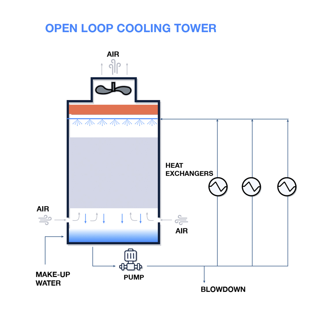
In general, there are two main types of systems in which pumps can be installed, open-loop and closed loop systems. Open-loop systems are circuits in which the pumped fluid is exposed to the local atmosphere at some point in the circuit. A typical open-loop system would be a cooling tower system where the flowpath is linear, i.e. fluid transfer between two vessels.
Get your pump selection right the first time. Free 14-day FluidFlow license.
Conversely, closed loop systems as the title suggests are closed piping circuits where the pumped fluid circulates in a closed loop without any exposure to the local environment and typically without transfer of fluid into or out of the closed loop.
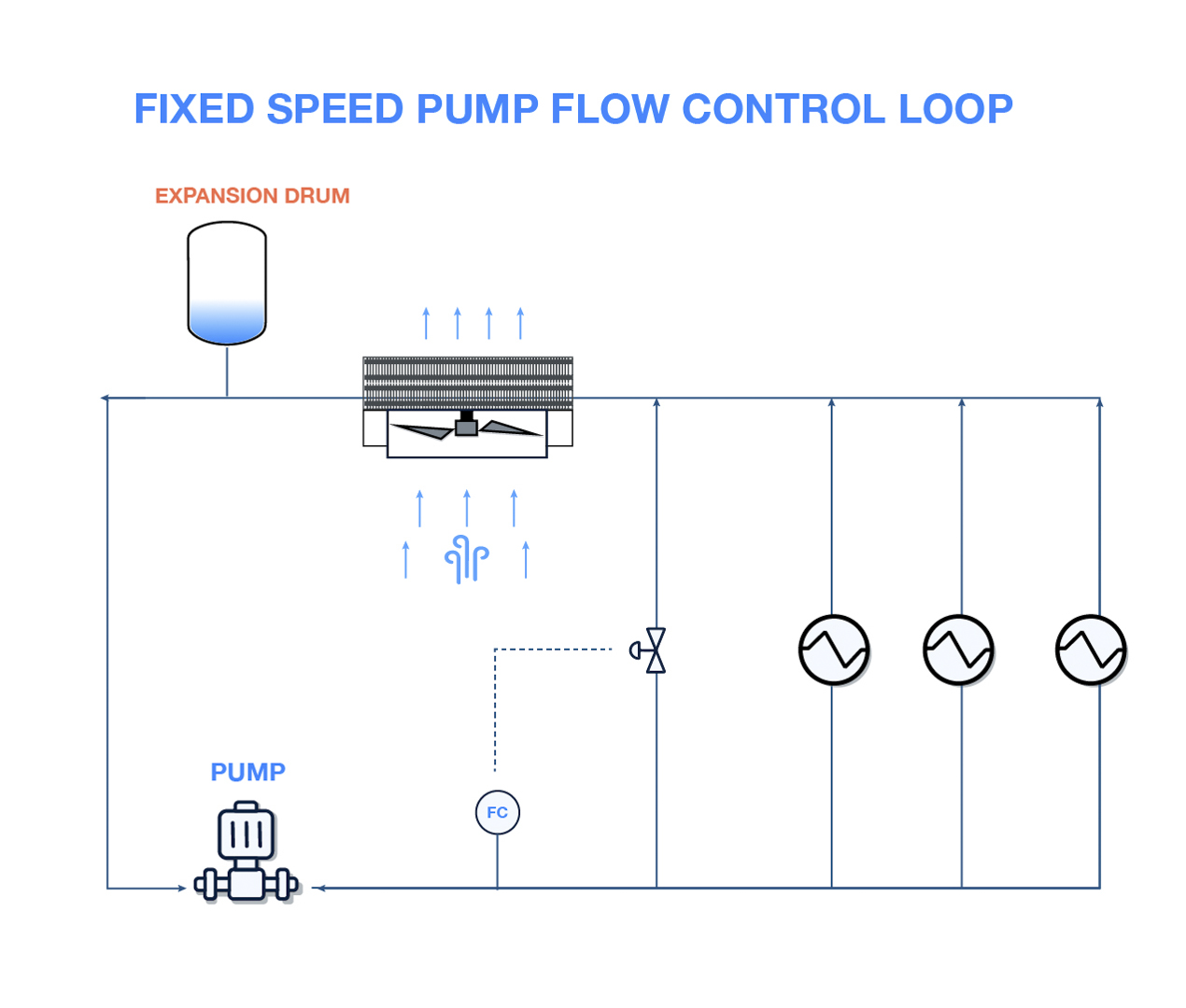
Examples of closed loop systems include hot oil circuits, cooling/chilled water systems, hot water heating and air conditioning systems. Figure 1 provides an illustration of a closed loop fresh water cooling system consisting of heat exchangers, circulating pumps, orifice plates and over 300 M of pipework.
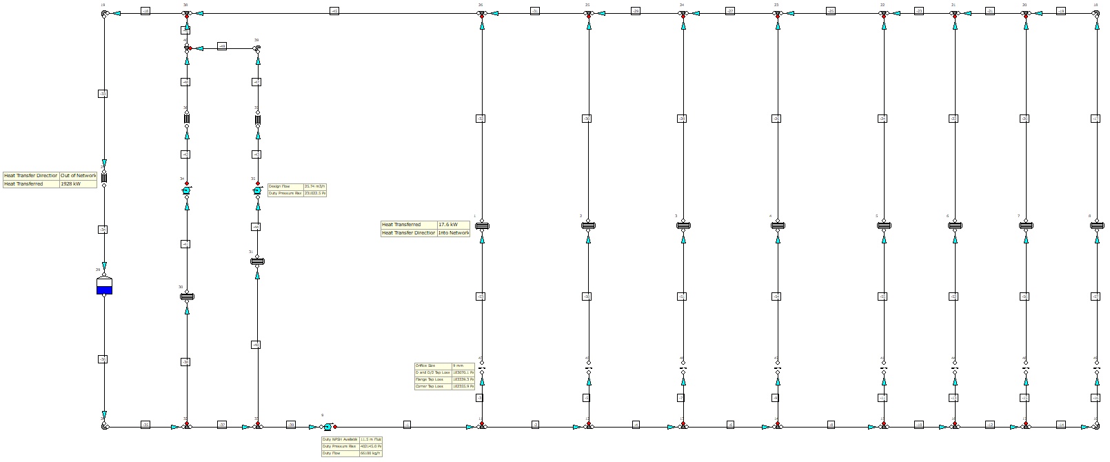
Figure 1: Closed Loop Fresh Water Cooling
One of the unique aspects of closed loop piping systems is that the static elevation is not accounted for in head-pressure calculations as these systems are largely unaffected by static pressure. However, just like open flow systems, we still need to make checks for sufficient NPSHa, that the static pressure throughout the system does not fall below the fluid vapor pressure and therefore induce cavitation etc. Any pump selected for the closed loop system must be able to transport the fluid to the highest point without flashing or inducing vacuum and the lowest point must also be evaluated for pump shut-off pressure. A closed loop circuit will exhibit only friction losses. Pumps operating in closed loop systems are therefore only required to overcome dynamic friction losses.
Let’s consider the operating conditions of a closed loop system with an elevation change of say, 10.0 M. The system circulating pump is required to transport the fluid from the bottom of the system (0 M) to the top at 10.0 M. It would initially appear that the pump must overcome the height difference of 10.0M however, due to gravitational effects, this isn’t the case as for every metre of fluid pumped vertically upwards, a corresponding 1.0 M of fluid drops on the return side of the system.
When the system is motionless, i.e. the fluid is not being circulated, the pump’s suction and discharge exhibit the same pressure exerted by the two separate 10.0 M columns of fluid which are connected at the top. An alternative way of considering this is, the suction pressure available at the pump is equal to the discharge pressure required to move the fluid to the top of the system.
Regardless of where the pump is positioned in the loop, the differential head developed by the pump will always be the same.
As you would expect, the head required to maintain flow in a closed loop system decreases as flow decreases and becomes greater as flow increases. In well-designed systems, the friction losses will decrease proportionally with a decrease in flow rate.
Large scale closed loop systems can become complex to manually design as they often have many multiple branch lines or sub-loops.
When selecting a constant speed centrifugal pump for closed loop systems, the best efficiency point (BEP) on the pump efficiency curve should fall between the design minimum and maximum flow points on the pump capacity curve. This ensures the pump operating efficiency is maximised across the expected pump operating conditions.
The performance curves shown in Figure 2 show that, the centrifugal pump achieves the maximum flow condition of 1400 m3/h at 55.0 M TDH and rises just 5.0 M at the minimum design flow rate of 700 m3/h. Note, the flow experienced in this sample system at any point in time is based on the demand of the system.
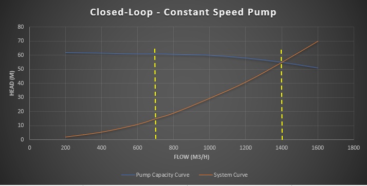
Figure 2: Closed Loop – Constant Speed Pump
Note, a “flat” pump capacity curve profile is preferred for closed loop systems with variable flow due to the energy savings which can be achieved at lower flow conditions.
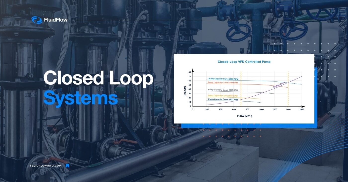
Although choosing a centrifugal pump with a “flat” capacity curve profile offers potential energy savings, much higher energy savings can be achieved by selecting a suitable VFD controlled pump (Figure 3). Since the system resistance curve reduces steadily from maximum to minimum flow (in this case 1400 to 700 m3/h), frequency control can be used to achieve the desired operating condition at low flow and in doing so, achieve much higher savings in comparison to that of a constant speed pump using valve throttling to adjust or regulate flow.
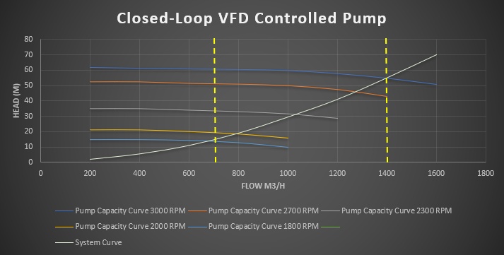
Figure 3: Closed-Loop – VFD Controlled Pump
The reason a much higher reduction in power is achieved by using the VFD pump is, a significant reduction in pump operating speed is achieved and secondly, the pump BEP efficiency isomer closely follows the system curve. As such, at 700 m3/h, the control frequency at the lower operating speed has almost the same efficiency as it does when the pump is operating at the speed required to achieve maximum flow.
If you are considering a VFD controlled centrifugal pump for an application, select the highest efficiency pump with a BEP that falls at or just to the left of the maximum flow condition. Keep head rise to minimum flow as low as the application will allow and test your pump selection using an appropriate software tool. This will allow you to evaluate the pump performance at different operating conditions.
References:
The Practical Pumping Handbook, Ross Mackay.
Pump Selection for VFD Operation, Joe Evans.
knowledge base
Ready to apply this in FluidFlow?
Build your first closed-loop model now — Modeling Closed Loop Systems in FluidFlow walks you through it step-by-step.