FluidFlow Software
Specification Sheet
FluidFlow is a comprehensive pipe flow simulation software that enables engineers to model, design, and analyze any liquid, gas, two-phase, slurry, or non-Newtonian piping system with proven accuracy and 80% time savings.
FluidFlow Information
| Full Product Name | Piping Systems FluidFlow (latest release v3.54) |
| Pricing per seat (annual) | Annual lease including SUM £3240 – £9990 per server seat per annum.For perpetual licensing including SUM from 2 seats upwards contact us |
| License Installation | Network License Installation Instructions |
| License Activation | Provided by us either manually or automatically, see instructions above |
| License Use Permitted | Global use included |
| Company Profile | Since its formation in 1984, Flite Software Ltd has been recognized worldwide as a quality supplier of engineering applications and selection software products. The company has specialized products for solving fluid flow design problems and has developed a state-of-the-art component-based technology for developing fluid equipment selection and configuration products.Our Mission Statement at Flite is to provide superior technology that enables engineers, specifiers, and designers to dramatically reduce design time whilst improving design quality.Piping Systems FluidFlow is the company’s main off-the-shelf product and offers a complete design environment for the hydraulic design, analysis, and troubleshooting of fluid systems. This product is used by thousands of engineers and designers throughout the world and in many varied types of applications. Anywhere you need to move fluids by pipe you can use FluidFlow.By combining engineering design skills with the latest software development techniques, Flite Software has created a flexible architecture of software components. The components can be easily utilized to produce complex rule-based product selections across a variety of platforms. This software architecture and modular design provide cost-effective, exact solutions for product selection “catalogs” and for integrating these solutions into existing workflow processes. |
| Location | Block E Balliniska Business Park, Springtown Road, Londonderry, Northern Ireland, BT48 0LY |
Software Details
| Software Overview | Complete Pipe Flow Simulation Software Model, design, or analyze any liquid, gas, two-phase, slurry or non-Newtonian pipe flow system from a single software solution. |
| Ease of Use – Intuitive user interface – Short learning curve – Save up to 80% of design time | |
| Calculation accuracy – Proven calculation reliability – Tested and verified against published data & real-world systems – Library of ‘Quality Assurance’ test models included | |
| Automatic equipment sizing – Powerful auto-sizing technology is included across all modules. – Automatically size: Pumps, Safety Relief Devices, Fans, Orifice Plates, and Control valves to industry standards. | |
| Thermal energy transfer – Heat Transfer functionality is included for all modules, as standard. – Ensure optimum energy efficiency on all of your designed systems. | |
| Type of Software | Hydraulic Calculation Software |
| Industry Applications | ∙ Aerospace ∙ Automotive ∙ Aviation ∙ Aviation Fuel Systems ∙ Chemicals ∙ Educational Institution ∙ EPC ∙ Equipment Manufacturer ∙ Fire Protection ∙ FMCG ∙ Mining & Metals ∙ Oil & Energy ∙ Paper Processing ∙ Pharmaceutical ∙ Pulp & Paper ∙ Research Body ∙ Semi-Conductor Manufacturer ∙ Shipbuilding ∙ Space Exploration ∙ Standards Agency ∙ Utilities |
| Language | FluidFlow is available in French, Spanish, and English.We can provide the tools to translate the interface to any language |
| Licensing | Annual, Quarterly, Perpetual, Named User *Trial Licenses require online login |
| Systems Modeled | |
| Liquids | via Liquid Module |
| Vapor | via Gas Module |
| Non-Newtonian | via Slurry Module |
| Two Phase Liquid – Vapor | via Two-Phase Module |
| Two Phase Liquid – Solid / Slurries | via Slurry Module |
| System Calculation | |
| Simple Systems | Yes |
| Advanced Fluid Networks | Yes |
| Flash / Phase Change Calculations | Yes |
| Phase Change Separation Calculations | Yes (For Liquid-Vapor Mixtures) |
| Transient Analysis | Coming soon |
| Customizable Calculations | Yes via Scripting Module (For “Light” Dynamic Analysis), Multi Calc functionality and Back Calc Input Tool (Reverse Calculation Feature) |
| Unit of Measurement (UOM) specification | Yes Two major selections only: SI and US Basic, there is an option to add preferred unit sets. Changing variable units is done individually per parameter in the Data Pallete and saving it as a new Environment. |
| Wide range of component and property databases | Yes FluidFlow contains a comprehensive database of 1,283 fluids enabling you to quickly model fluid transportation systems. |
| Customizable component and property databases | Yes Users can choose from five options when adding new fluid to the Database: 1) Simple Newtonian 2) Pure Newtonian 3) non-Newtonian Liquid 4) Gas (No Phase Change) 5) Petroleum Fraction or Crude |
| Pipe Database | Yes FluidFlow contains a database of standard pipe sizes that can be used when building a network. FluidFlow supports the following pipe database: 1) Acrylonitrile-Butadiene-Styrene ABS Pipe 2) Aluminium Pipe or Duct 3) Asbestos Cement Pipe 4) Cast Iron Pipe 5) Concrete Pipe 6) Copper Pipe 7) Ductile Iron Pipe 8) Flexible Smooth or Corrugated Hose 9) Glass Pipe 10) Polyethylene (PE) Pipe or Duct 11) PolyVinylChloride (PVC) Pipe or Duct 12) PP or PFA Pipe or Duct 13) Stainless Steel Pipe or Duct 14) Steel Pipe or Duct |
| Customizable pipe database | Yes The user can also supplement the pipe database by adding new pipe size data for specific applications. |
| Heat Transfer Functionality | Yes FluidFlow includes heat transfer functionality on ALL modules. Engineers can study heat transfer effects at heat exchangers, pipes, and junctions. FluidFlow can model shell and tube exchangers, plate exchangers, coils, and autoclaves. Users can choose from a range of heat transfer options: a) Buried pipe calculations. b) Pipe heat loss/gain calculation. c) Fixed heat transfer rate. d) Fixed temperature change. e) Ignore heat loss/gain. |
| Losses in fittings Calculation Method | The fitting resistance K is calculated by FluidFlow using the following methods: a) Idelchik (more accurate compared to Crane) b) Miller (more accurate compared to Crane) c) Craned) SAE FluidFlow contains a database of General Resistance elements that can be used to represent any fitting or device when building a network. The user can also supplement this database by adding new resistance elements and values. |
| Input for pump curve function | Yes Pump performance data can be entered into a FluidFlow model by one of the following methods: 1) Manual data entry 2) Pump curve database based on multiple pump vendors. |
| Input for control valve Cv values/Cv curve function | Yes |
| Applicable to Factor Method | Yes |
| Applicable to Isometric Method | Yes |
| Scenario Manager | None. Users need to save an additional file to create a new case/scenario. V3.52 includes Multi-Calc |
| Calculation Results | – Configurable MS Excel results table – Can generate Bill of Materials summary report – Can generate reports in English, French, and Spanish |
| Calculation Alerts, Warnings, and Hints | Up to 118 calculation design alerts, warnings, and hints Liquid, Vapor, and Two-phase Velocity limits (Minimum and Maximum) and Control valve opening (Minimum and Maximum) can be configured to generate warning criteria |
| Troubleshooting | FluidFlow’s Help Section discusses some useful modeling hints and tips to aid in troubleshooting. |
| Data Management | – JSON format support for database editors – FlowDesigner compatibility for file exports – PCF enhancements for pipe diameter and length properties – Improved Hydrogen by including NIST Density Estimation in the database (version 3.53) |
| UI Toolbar and Navigation | – Split flowsheet toolbar into Flowsheet Tools and Flowsheet Settings – Separate dockable Input Editor window from the Data Palette – Enhanced filter capabilities for Messages and Results lists – Improved graphic objects with additional customization options |
Model Elements
| Boundaries | – Pressure – Flow – Tank or Vessel Reservoir (Either source or destination only) – Atmospheric Ends (Sprinkler or Customized atmospheric discharge ends) |
| Pipes | – Pipes (Standard) can be modelled – Rectangular or Annulus can be modelled – Hose (Flexible or Corrugated) can be modelled – Can automatically size pipe via established Criteria (Economic velocity (using Generaux equation), Standard velocity, or Pressure gradient) pipe scaling can be applied to consider pipe degradation or current status of existing systems – Heat Effects on the pipe can be ignored or can be calculated – Heat Effects on the pipe can be modeled as fixed temperature change, fixed – Heat transfer rate, or buried pipe |
| Junctions – Pumps | – Can autosize pump based on desired flow or pressure rise – Pump curves from several vendors already available on the default database – Heat loss/gain models can be customized on the pump – Slurry pump solids derating can be modeled using Fixed Reduction, King or HI guidelines |
| Junctions – Compressor / Blowers / Fans / Turbines | – Can autosize compressors or blowers based on desired flow or pressure rise – Compressor, Fan or blower curves from several vendors already available on the default database – Heat loss / gain models can be customized |
| Junctions – Fittings | – Can model connectors (no resistance), bends, mitre bends, tees, symmetric Y-junctions, cross junctions – Bends and mitre bends can be modeled based on angle and defined as Idelchik, Miller, Crane, or SAE – R/D ratio for bends can be customized Heat loss/gain across bends for these fittings can be modeled – Can model area size changes for reducers and expanders including abrupt size changes, venturi’s, and in-line nozzles – In-line nozzle model can apply Long radius or ISO 5167 equations – Orifices can be modeled as thin or thick plates using ISO 5167 equations |
| Junctions – Valves | – Default database enables modelling of butterfly, diaphragm, ball, gate, globe, ball float, plug, pinch, Y-globe, needle, slide valve, penstock, 3-way and fire hydrant – Default database also available for different check valve types: swing check, tilting disc, piston operated, spring loaded, foot operated – Valve % opening can be customized from 0 – 100% in infinite increments – Several valve models availabe in the valve database – R/D ratio for bends can be customized – Heat loss/gain across valves can be modelled |
| Junctions – Control Valves | -Can model constant upstream and downstream pressure control valves via self-acting pressure reducer or sustainer element or via pressure control valve – Can model flow control valves – Flow or pressure control valve type can be selected when sizing – Separate element for Gas control valves – Default database available for several control valve vendors – Heat loss/gain can be modeled |
| Junctions – General Resistance | – Can model pressure loss constants in “K”, “Kf” or “Kv” values – Default elements for some specialized components such as Inline filter, Packed bed, cyclone, Labyrnth seal, Centrifuge, expansion join / stuffing box, cols, tube bundles, constant head loss are available – Generic element for user defined general resistance available for the model using a polynomial input – Heat loss/gain across can be modelled |
| Junctions – Relief Valves | – Can model relief valve or rupture discs in Autosize on or Rating (Autosize off) mode – Relief device (valve or disc) calculations can be set to utilize either API RP 520 or ISO 4126-1 equations – Relief Valve set pressure can be configured to MAWP of 10% (Sole Device), 16% (Multiple Device) and 21% (Fire) – Default database available for several Relief Valve vendors – Default values for Rupture disc Kd (Discharge coefficient) available for Sharp edge, bellmouth, in-projecting, API or liquid Heat loss/gain across can be modelled |
| Junctions – Heat Exchangers | – Can model hydraulic considerations for Shell and Tube (S&T) and Plate and Frame (P&F) Heat Exchangers – Pressure drop model HX can be determined using tube (S&T) or plate (P&F) details or via polynomial expression using Vendor pressure drop data or a fix value can be applied – Vaporization / phase separation can be modelled using Knockout pot element – Temperature increase can be modelling using jacketed vessel element – Heat loss/gain across can be modelled |
Liquid, Incompressible Flow
| Product Description | Delivers fast and accurate design for Newtonian fluids.Determines system operating pressures, flow distribution, and fluid physical properties.Allows for the modeling of a wide range of line equipment items. |
| Physical Property Correlation | User-defined Liquid properties can be fixed (for simple Newtonian), based on temperature correlation data or Pure Newtonian via various equations of state (Peng-Robinson, Lee-Kesler, and Benedict-Webb-Rubin-Han-Starling). |
| Pressure Drop Correlation | FluidFlow solves the fundamental conservation equations of mass, energy, and momentum. Users can choose from four pipe pressure loss models as follows; 1) Moody (Darcy-Weisbach) 2) Hazen Williams 3) Fixed Friction Factor (Darcy) 4) Shell – MIT |
| Calculates incompressible (liquid) network pipe systems. | Yes |
| Calculates systems that are pressure driven | Yes |
| Calculates systems that are gravity driven | Yes |
| Calculates systems that are pump driven | Yes |
Gas, Compressible Flow
| Product Description | – Accurate for both low and high-velocity gas flow systems. – Solves the conservation equations and an equation of state ensuring an accurate solution. – Auto-detection of choked flow conditions. |
| Physical Property Correlation | User-defined vapor properties can be No phase change gases based on temperature correlation data or Pure Newtonian via various equations of state (Peng-Robinson, Lee-Kesler, and Benedict-Webb-Rubin-Han-Starling). Hydrogen includes NIST Density Estimation. |
| Pressure Drop Correlation | FluidFlow uses a calculation procedure that solves the conservation equations and an equation of state for small pressure loss increments. This means FluidFlow obtains a much more rigorous and accurate solution reflective of actual plant performance. Available equations of state include Benedict-Webb-Rubin-Han-Starling, Peng-Robinson, and Lee-Kesler.Using the EOS the gas thermophysical properties such as enthalpy and density are calculated as the gas accelerates. FluidFlow makes no assumptions of gas ideality or adiabatic flowing conditions.FluidFlow algorithm dynamically splits the pipe into segments based on an incremental density change. The method is a development of a paper originally published in The Chemical Engineer – Relief Line Sizing for Gases Part1 and 2. Dec 1979 – HA Duxbury. |
| Calculates compressible network pipe systems | Yes |
| Accurately models real gases | Yes |
| Accurately models heat transfer | Yes |
| Accurately models highly compressible (sonic and near sonic) system | Yes |
Two-Phase Flow
| Product Description | – Automatically track fluid phase-state, performs flash calculations, liquid holdup calculations and develops flow regime maps for each pipe segment. – Highly accurate results were developed using a “marching” solution algorithm. |
| Physical Property Correlation | – Users can perform Fluid mixing on the software using database fluids with Physical properties based on Standard Mixing Rules – Two-phase properties are determined for either Pure Newtonian or Fluid mix via estimate such as Heat of vaporization (can also be based on Literature) surface tension (via linear function or estimation) |
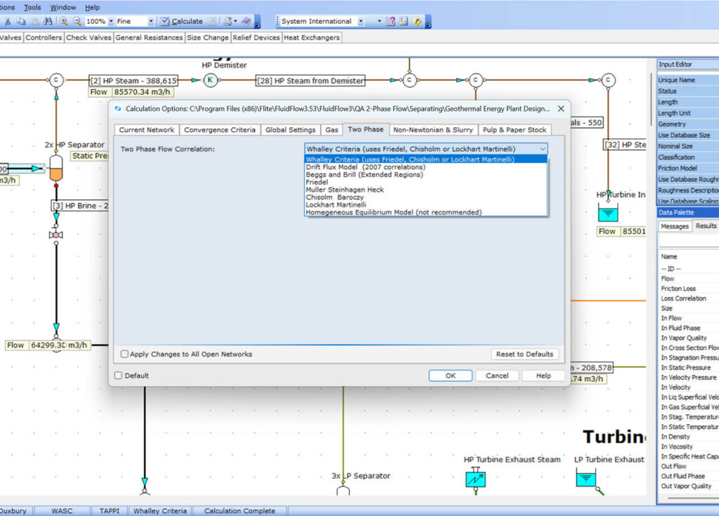
| Pressure Drop Correlation | FluidFlow can be used to model fixed or changing vapor quality systems with heat transfer included. The calculation method includes eight (8) two-phase correlation methodologies: 1) Whalley Criteria (uses Friedel, Chisholm, or Lockhart-Martinelli) 2) Drift Flux Model (2007 correlations) 3) Beggs and Brill (Extended Regions) 4) Friedel 5) Muller-Steinhagen and Heck 6) Chisholm Baroczy 7) Lockhart-Martinelli 8) Homogeneous Equilibrium Model |
| Flow Regime maps | Yes |
| Calculates two-phase flow network pipe systems | Yes |
| Calculates the change in vapor fraction across the piping length | Yes |
Slurry & non-Newtonian Flow
| Product Description | – The Slurry Module can be used to model settling, non-settling, non-Newtonian fluids and Pulp & Paper Stock flow systems. – Analyze liquid-solid flow systems for mineral hydro transport, metal concentrate pipelines, tailings, paste backfill systems, dredging, wastewater treatment and more – The industry choice for designing, troubleshooting and optimizing slurry flow systems. |
| Physical Property Correlation | – Four (4) rheology models for non-Newtonian viscosity behavior (Power Law, Bingham Plastic, Casson and Herschel Bulkley), the yield stress can be calculated or specified, and R² coefficient is available for accuracy – Expandable database with default data for common non-Newtonian liquids and solid physical properties for at least 11 common materials for metals processing, coal, and sands handling. – Sixteen (16) pulp type options for TAPPI Method – Definable Moller K pulp property data |
| Pressure Drop Correlation | – Specific empirical friction loss methods applied for each non-Newtonian viscosity model (Darby, Chilton-Stainsby, Converted Power Law) – Wide selection of industry accepted and latest settling slurry friction loss correlations 1) Vsm Model 2) V50 Model 3) Four Component Method (4CM) 4) Durand 5) Wasp 6) WASC (Wilson-Addie-Sellgren-Clift) Method 7) Sellgren–Wilson Four-Component Model 8) Liu Dezhong – Configurable pressure loss correlation options for vertical piping: 1) Vertical Pipe WASC Loss 2) 4CM 3) Spelay, Gillies, Hashemi and Sanders 2017 Collisional Stress Model – Moller K and TAPPI Pulp and Paper Stock Pressure Loss Correlation |
| Deposition Velocity Modeling | – Configurable methods for maximum deposition limit velocity modelling: 1) WASC (Wilson-Addie-Sellgren-Clift) Generalized Relationship 2) As a function of particle size 3) GIW VSCALC – Configurable methods for maximum deposition limit velocity correction for non-horizontal flows: 1) Wilson – Tse 1984 Chart 2) Extended Wilson – Tse 1984 Chart – Calculation and reporting of slurry characteristic velocities such as: – Oroskar and Turian Critical Velocity – Schiller and Herbich Minimum Velocity – Maximum deposition limit velocities for Wilson–GIW, Thomas 1979, Thomas 2015 and Wilson 1992 Models |
| Centrifugal pump performance modeling | – Configurable performance adjustment methods for non-Newtonian viscosity effects and solids friction loss at pump internals: 1) RP King 2) HI Guidelines 3) ANSI 2021 Monosize 4) GIW 4CM 5) Fixed Deration |
Experience FluidFlow Today
What’s Included in your Free Trial:
Full Professional Features
Access to all simulation modules and advanced tools
14 full days
Plenty of time to test with your real projects
Sample Projects Included
Pre-built examples to get you started immediately
Live Support During Trial
Get help from our engineering team via chat and email