Gas Flow Simulation Software
FluidFlow Compressible Gas Analysis
Model Compressible Gas Flow Across Pipe Networks
Gas doesn’t behave like a liquid. As pressure drops along a pipeline, gas density falls, velocity rises, and friction resistance intensifies — all at once, all coupled. FluidFlow solves this with a rigorous compressible flow solver engine, giving you accurate pressure drop results across gas networks of any complexity, without manual workarounds or simplified assumptions.
The Problem with Ideal Gas Shortcuts
Most single-line gas flow formulas assume constant properties or ideal gas behavior. That works for rough estimates on simple systems. It breaks down when:
- Pressure ratios are high — density changes significantly from inlet to outlet, making a single-point calculation inaccurate
- Networks branch and recombine — flow distribution across headers depends on coupled pressure and velocity changes at every junction
- You’re near sonic conditions — choked flow limits capacity in ways that no fixed-property formula can predict
- Real gas deviation matters — at elevated pressures or low temperatures, Z-factor deviates meaningfully from 1.0, and ideal gas assumptions introduce systematic error
FluidFlow is built to handle all of these cases in a single unified model.
How FluidFlow Models Compressible Gas Flow
1. Establish Gas Physical Property
Select your gas from the fluid database — air, natural gas, nitrogen, steam, or a custom mixture. The built-in database covers the gases most commonly encountered in industrial piping applications, and it is designed to be extended: if your project involves a gas not yet in the database, you can define a custom fluid by entering the key transport properties directly.
For every fluid in the database, FluidFlow models gas properties using Equations of State (EOS) — mathematical models that relate pressure, temperature, and composition to density and other thermodynamic properties, capturing real gas behavior rather than relying on ideal gas assumptions.
2. Define your gas and network
Assign boundary conditions: known pressures, known flow rates, or compressor performance curves. Known pressure boundaries are best suited for capacity questions — the solver calculates how much flow the network can deliver at the specified supply pressure. Known flow boundaries are ideal for distribution studies, where total throughput is fixed and the focus is on how flow splits across branches and headers. Compressor performance curves can be entered directly as supply conditions, allowing FluidFlow to find the operating point where the compressor curve intersects the network resistance.
3. Solve the network with the Duxbury method
FluidFlow calculates gas friction pressure drop using the Duxbury incremental marching method — an approach specifically designed for compressible flow with real gas behavior taken into account. Rather than applying simplifying assumptions like some competitors apply, FluidFlow’s solver divides each pipe into fine internal segments and marches along the flow path, updating pressure, temperature, density, and velocity at each step using real-gas equations of state.
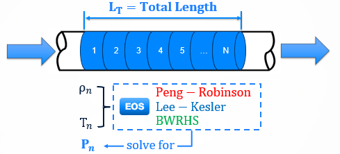
This captures the full compressible flow cascade:
- Pressure drops → density decreases → velocity rises → friction resistance increases
- Each segment feeds accurate conditions into the next
The result: accurate pressure drop predictions across the full network, even for long high-pressure pipelines with large pressure ratios.
3. Inspect profiles and constraints
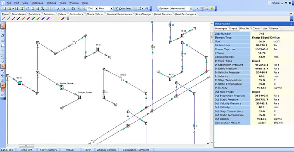
FluidFlow reports inlet and outlet conditions for every pipe segment:
- Static and stagnation pressure
- Gas density, velocity, and Mach number
- Temperature (including Joule–Thomson cooling effects)
- Flow distribution
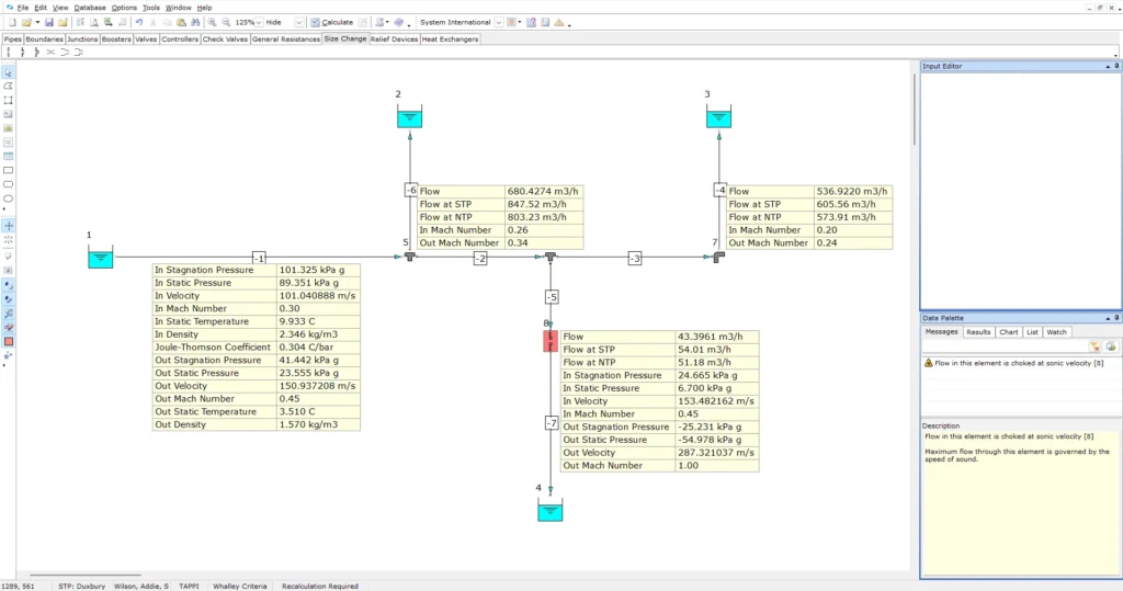
Choked flow warnings are flagged automatically wherever sonic conditions are approached or reached.
Key Capabilities
Real-gas property handling
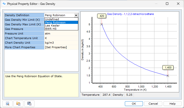
Gas density is calculated from pressure and temperature at every point in the network using any of these equations of state:
- Peng – Robinson
- Benedict – Webb – Rubin – Han -Starling (BWR – HS)
- Lee – Kesler
- NIST (For Hydrogen)
The compressibility factor Z is recalculated continuously along the flow path — there is no ideal gas assumption applied.
Choked flow detection
FluidFlow automatically detects when flow approaches or reaches sonic velocity and issues explicit warnings. These three distinct choking types can be easily identified:
- Endpoint choking — pipe discharge to the atmosphere or a large vessel
- Restriction choking — orifices, control valves, nozzles
- Expansion choking — small-to-large area transitions and branch-to-header junctions
Mach numbers are reported at pipe inlets and outlets for every segment, enabling rapid identification of the limiting element in any network.
Joule–Thomson temperature tracking
When gas expands through restrictions or along pipelines, temperature drops — even without external heat transfer. FluidFlow includes the Joule–Thomson effect by default, ensuring temperature profiles reflect actual thermodynamic behavior. This is critical for:
- Identifying hydrate formation risk in natural gas systems
- Checking downstream temperatures against material design limits
- Sizing heat tracing or pre-heating requirements at pressure letdown stations
Tee junction modeling for gas headers
Flow distribution in gas headers is driven by the interaction of header velocity, density change, and branch vs. run pressure losses at each tee. FluidFlow computes tee losses using multiple industry methods (Idelchik, Miller, SAE, Crane) and accounts for the velocity-ratio and diameter-ratio effects that govern branch flow resistance. This enables accurate analysis of fishbone distribution headers, parallel flow paths, and multi-takeoff gas systems.
Why FluidFlow
No simplifying flow assumptions
FluidFlow does not apply isothermal or adiabatic flow assumptions to simplify the calculation. Real-gas equations of state and the Duxbury marching method are applied to every gas pipe, regardless of pressure ratio or network complexity.
Boundary condition flexibility
Specify known pressure or known flow at any network boundary. Use compressor performance curves as supply conditions. Mix boundary types across a single network to match the real operating constraints of your system.
Defensible, auditable results
Every result traces back to explicit inputs: gas properties, pipe geometry, boundary conditions. Inlet/outlet conditions are reported at the component level, so pressure profiles and flow distributions can be reviewed and validated against field data or hand calculations.
Use Cases
- Gas transmission and distribution networks — pressure drop analysis, flow capacity checks, and operating point evaluation for pipeline systems
- Process gas headers — flow distribution analysis for multi-branch headers feeding reactors, furnaces, or process equipment
- Flare and vent headers — back-pressure calculation, choked flow screening, and capacity verification for relief discharge systems
- Compressed air systems — distribution uniformity analysis, noise velocity screening, and balancing for industrial plant air headers
- Pressure letdown stations — Joule–Thomson temperature profiling and heat duty estimation for pressure reduction systems
- Gas turbine and compressor inlet/outlet networks — static vs. stagnation pressure handling for high-velocity ducting
- HVAC and ventilation systems — pressure drop and flow distribution analysis across duct networks, with direct support for square and rectangular conduit geometries alongside circular ducting
Frequently Asked Questions
Yes. Gas density is calculated using any of these equations of state, not the ideal gas law:
- Peng – Robinson
- Benedict – Webb – Rubin – Han -Starling (BWR – HS)
- Lee – Kesler
- NIST (For Hydrogen)
FluidFlow calculates Mach numbers at pipe inlets and outlets for every gas pipe and issues explicit warnings when sonic conditions are approached or reached. Three types are detected: endpoint choking (discharge to atmosphere), restriction choking (valves, orifices), and expansion choking (area increases). No manual threshold monitoring is required.
FluidFlow uses the uxbury incremental marching method for compressible gas pressure drop. The pipe is internally divided into fine segments, and properties are updated at each step using real-gas equations of state. No isothermal or adiabatic simplifying assumptions are applied.
Yes. FluidFlow supports gas, liquid, slurry, and two-phase flow in a single model. Different fluid types can coexist in the same flow sheet.
FluidFlow reports mass flow, actual volumetric flow, and standard volumetric flow (STP or NTP) for every component. Standard and mass flow are conserved at junctions; actual volumetric flow varies with local pressure and temperature. The reference convention (STP at 15 °C or NTP at 0 °C) is configurable per project.
Start Modeling Compressible Gas Networks
Download FluidFlow today
Accurately model compressible flow, predict pressure drop, and detect sonic choking, bottlenecks, and system limitations.
Questions?
Contact [email protected] or call +44 28 7127 9227.