Darcy-Weisbach Equation Explained | Pipe Pressure Drop Calculator

Darcy-Weisbach Equation: Calculating Pressure Drop in Pipes

The Darcy-Weisbach equation is the standard method for calculating frictional pressure drop in pipe flow. It applies to any Newtonian fluid, any pipe material, and any flow regime. Most other pressure drop methods are either simplifications of Darcy-Weisbach or limited to specific fluids.

This page covers the equation, how the friction factor is determined, when it applies, and how FluidFlow uses it within pipe network models.

---

The Equation

The Darcy-Weisbach equation relates frictional pressure drop to pipe geometry, fluid properties, and flow velocity:

Pressure drop form:

ΔP = f × (L/D) × (ρV²/2)

Head loss form:

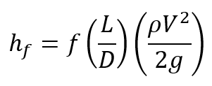
Symbol	Description	Units
ΔP	Frictional pressure drop	Pa
h_f	Friction head loss	m
f	Darcy friction factor	dimensionless
L	Pipe length	m
D	Inside diameter	m
ρ	Fluid density	kg/m³
V	Mean flow velocity	m/s
g	Gravitational acceleration	9.81 m/s²

The equation is straightforward once you have the friction factor. The friction factor is where the complexity lives.

---

Friction Factor: The Core of the Calculation

The Darcy friction factor depends on two things: the Reynolds number (flow regime) and the roughness of the pipe wall.

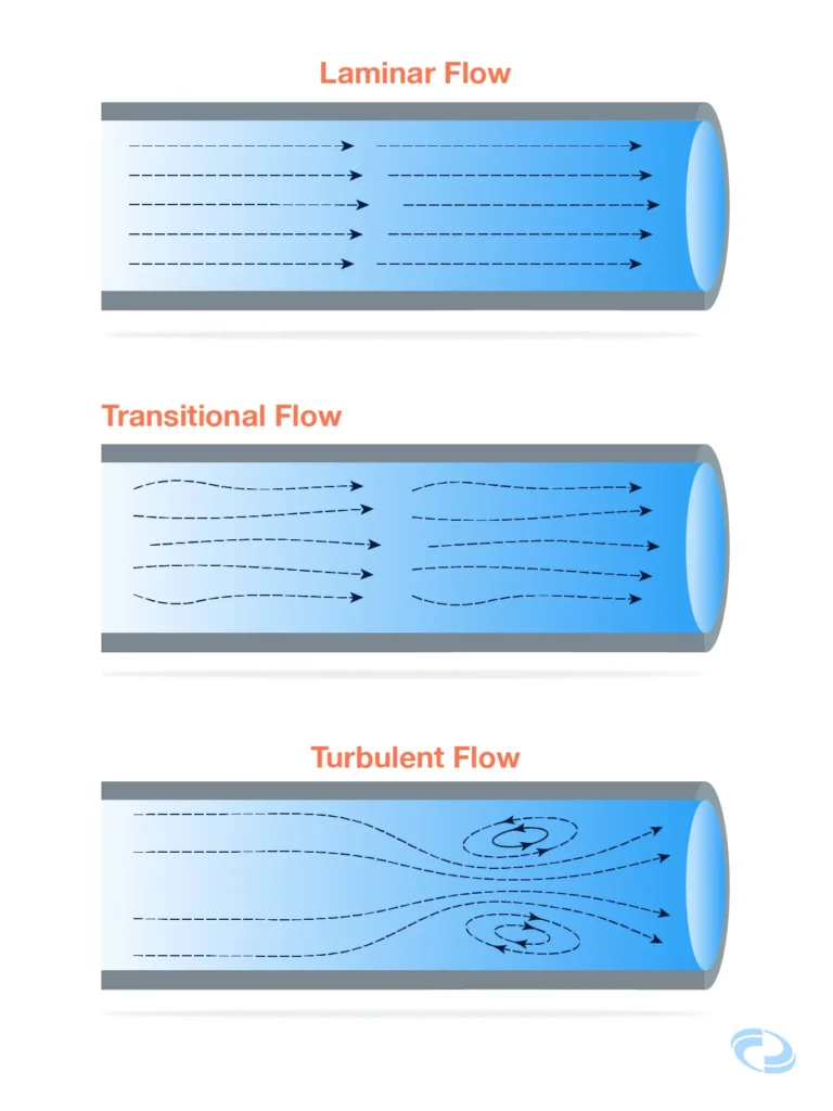
Reynolds Number

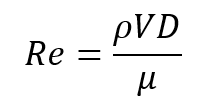
Re range	Flow regime
< 2,300	Laminar
2,300 – 4,000	Transition
> 4,000	Turbulent

Note: Tables above are based on typical published literature, actual Reynolds number range to demarcate laminar, turbulent and transition flow may vary according to experience.

In laminar flow, the friction factor has a simple closed-form solution:

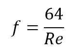
Pipe Roughness has no effect in laminar flow. The fluid layers slide over each other without interacting with the wall texture.

Turbulent Flow: Colebrook-White Equation

In turbulent flow, the friction factor depends on both Reynolds number and relative roughness (ε/D). The Colebrook-White equation captures this:

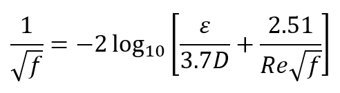
This equation is implicit — the friction factor appears on both sides. It cannot be solved algebraically. Engineers historically used the Moody chart (a graphical representation of Colebrook-White) to look up friction factors. FluidFlow solves this equation iteratively.

Symbol	Description
ε	Absolute pipe roughness (m)
ε/D	Relative roughness (dimensionless)

Pipe Roughness: Pipe Material Matters

The ratio of wall roughness to pipe diameter determines how much the wall texture affects friction. Common roughness values:

Pipe material	Typical absolute roughness ε (mm)
Drawn steel/copper	0.0015 – 0.002
Commercial steel	0.045
Cast iron	0.26
Concrete	0.3 – 3.0
PVC/PE (plastic)	0.0015 – 0.007
Corrugated/flexible hose	1.0 – 3.0

Smaller pipes have higher relative roughness at the same absolute roughness, so friction effects are proportionally larger in small-bore piping.

Pipe Ageing

Pipe roughness is not fixed. In service, pipe walls degrade over time, and the effective absolute roughness ε increases beyond the as-new values for any given material. This directly raises the Darcy friction factor and increases pressure drop for the same flow conditions. Common causes include:

• Corrosion — oxidation of metallic pipe walls (common in unlined carbon steel and cast iron)
• Scale and mineral deposits — calcium carbonate and other minerals precipitate from water and build up on the pipe wall
• Biological fouling — microbial growth in water and process systems creates a roughened biofilm layer
• Erosion — high-velocity or slurry flow can alter surface texture over time

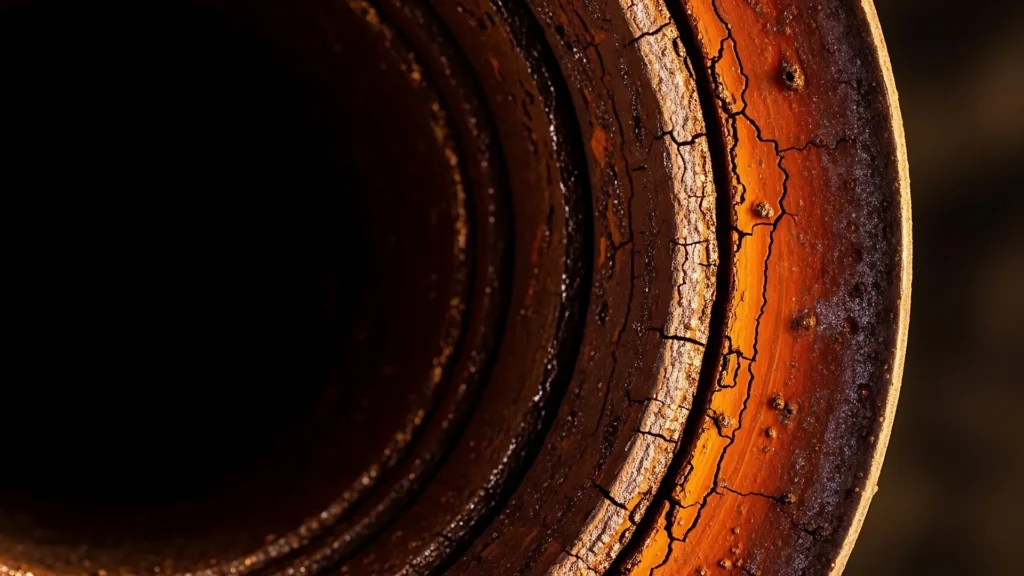
All of these mechanisms increase the effective absolute roughness ε, which raises the friction factor and increases pressure drop for the same flow rate.

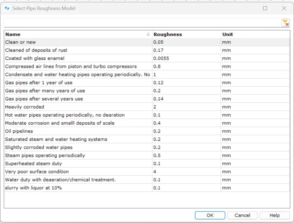
How FluidFlow handles pipe ageing: FluidFlow handles this by varying the absolute roughness value assigned to a pipe. Each pipe material in FluidFlow has its own database of pipe roughness values, giving engineers a range of options to choose from. For aged pipe conditions, engineers can select roughness value from that material’s database — or enter a custom value directly — to reflect the pipe’s actual condition rather than its as-new state. This can be applied on each pipe component, allowing engineers to accurately model networks where ageing and degradation vary across different sections of the system.

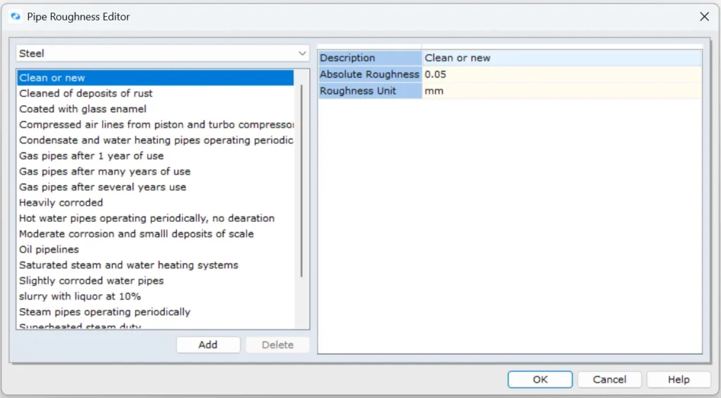
When assessing an existing system, using as-new roughness values will underestimate pressure drop and may lead to undersized pumps or incorrectly predicted flow distribution. Selecting a roughness value that reflects the pipe’s actual condition produces a more representative hydraulic model.

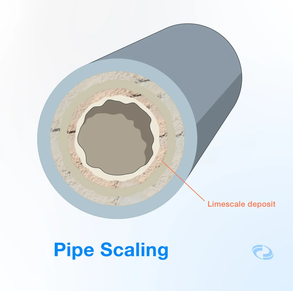
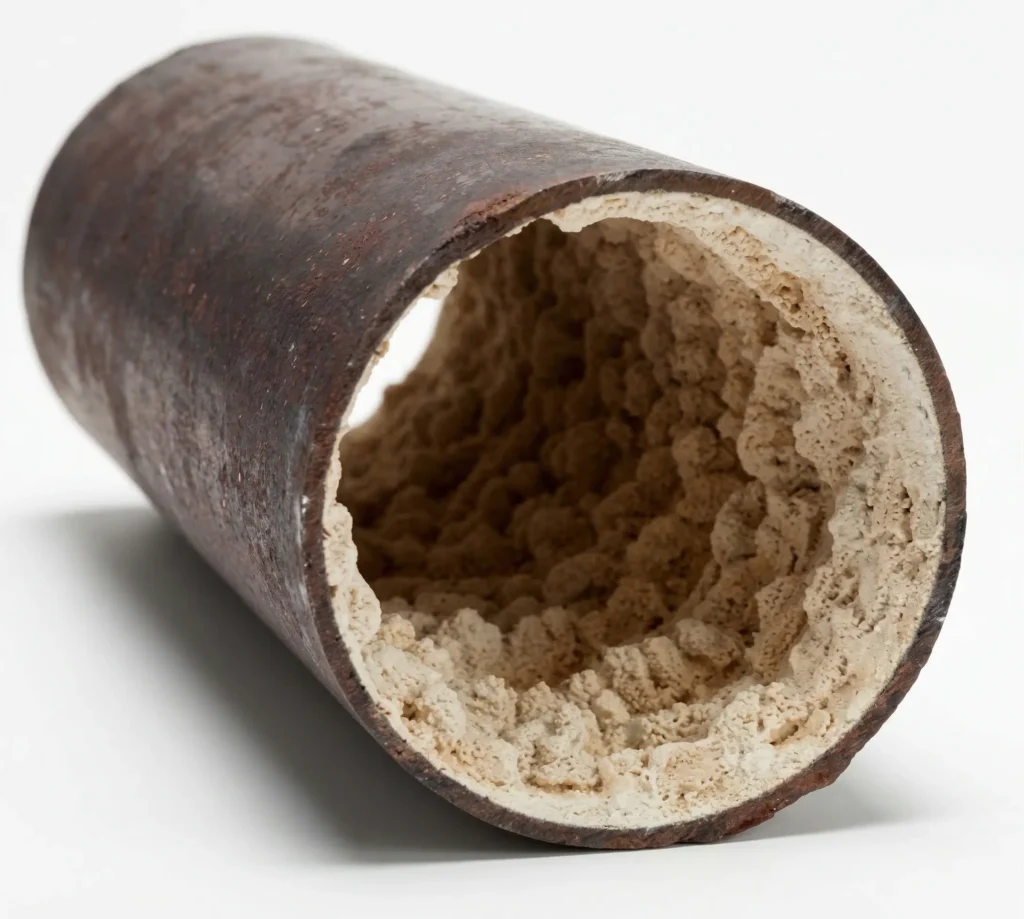
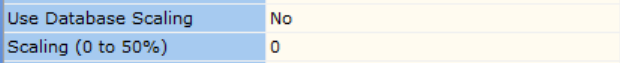
Pipe Scaling

Pipe scaling is a distinct phenomenon from wall roughness ageing. Scale deposits — typically calcium carbonate, calcium sulphate, or other mineral precipitates — build up on the inner wall of a pipe over time. Unlike surface roughness changes, significant scale deposits physically reduce the pipe’s effective internal diameter. This has two compounding effects on pressure drop: the smaller bore increases flow velocity at the same flow rate, and the Darcy-Weisbach equation amplifies both effects through the L/D term and the velocity-squared relationship.

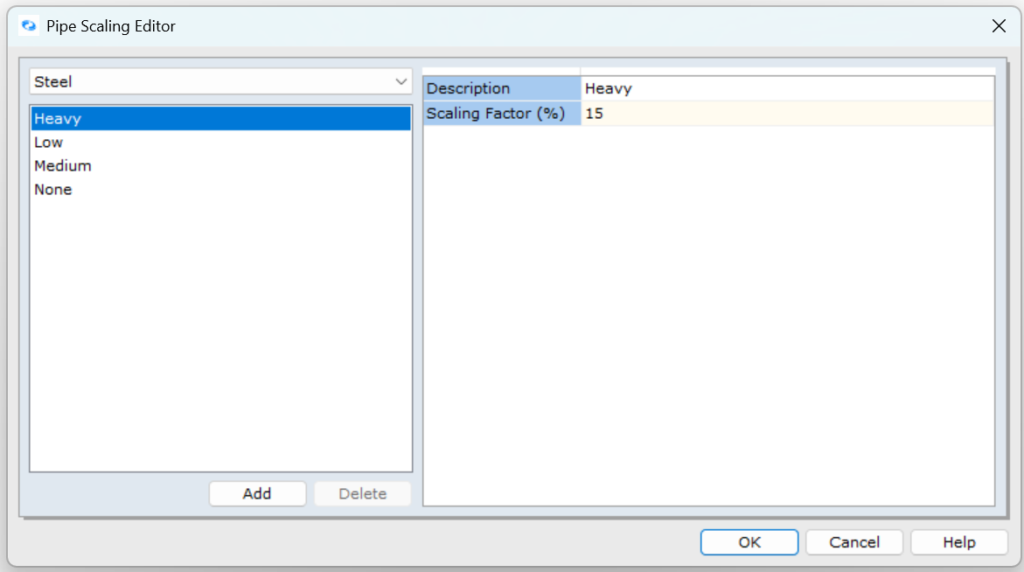
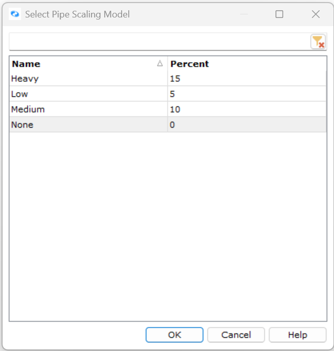
How FluidFlow models pipe scaling: FluidFlow models pipe scaling by applying a scaling factor that reduces the effective internal diameter used in the hydraulic calculation, without modifying the nominal pipe specification. FluidFlow includes a scaling database with predefined scaling values that engineers can select from — and, similar to how pipe roughness is handled, user-defined scaling values can also be entered directly to represent site-specific or measured conditions. The scaling value can be assigned on a pipe-by-pipe basis, enabling realistic assessment of partially scaled networks where deposit buildup is not uniform across the system.

---

When Darcy-Weisbach Applies (and When It Doesn’t)

Darcy-Weisbach applies to:

• Any Newtonian liquid at any velocity
• Any pipe material and diameter
• Laminar and turbulent flow
• Single-phase flow

It does not directly apply to:

• Non-Newtonian fluids — these require modified friction correlations (Power Law, Bingham Plastic, Herschel-Bulkley, Casson models). See non-Newtonian fluids.
• Compressible gas flow — gas density changes along the pipe as pressure drops. Rigorous gas flow calculation requires solving conservation equations with an equation of state, not a fixed-density Darcy-Weisbach approach.
• Two-phase flow — gas-liquid mixtures require specialized correlations that account for phase interaction.
• Open channel flow — Darcy-Weisbach applies to full-pipe (pressurised) flow only. Free-surface flow in open channels requires hydraulic radius-based methods (e.g. Manning’s equation).

---

Method	Notes
Idelchik	Extensive empirical foundation
Miller	Precise internal flow junction modeling
Crane	Simplified, practical, and widely referenced
SAE	Specialized modeling for aerospace and high-velocity systems

---

Other Pressure Drop Methods

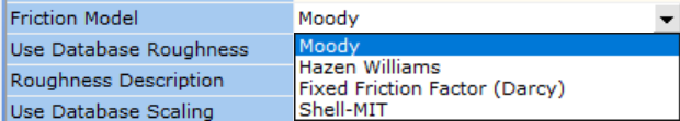
Darcy-Weisbach is the most general method, but it is not the only one. FluidFlow provides four liquid pressure drop models:

Method	Best for	Limitations
Moody (Darcy-Weisbach)	Any Newtonian liquid, any regime	Requires friction factor iteration in turbulent flow
Hazen-Williams	Water distribution systems	Only valid for water near 15°C, turbulent flow only
Fixed Friction Factor	Known or specified friction conditions	User provides the friction factor directly
Shell-MIT	Pipeline applications, viscous oils	Developed for oil industry applications

Darcy-Weisbach (Moody) is the default in FluidFlow because it is the most broadly applicable. Hazen-Williams is common in water utility work because the C-factor is simpler than iterating Colebrook-White, but it only works for water in turbulent flow.

---

How FluidFlow Uses the Darcy-Weisbach Equation

In FluidFlow, pipe friction is one of several contributors to the total pressure drop calculated across each pipe segment. The solver combines the Darcy-Weisbach friction component with fitting losses (calculated using K-factor correlations for valves, bends, tees, and other fittings), static head from elevation changes, and pressure contributions from equipment such as pumps, control valves, and heat exchangers. These are summed up to establish the local pressure balance. FluidFlow then solves the entire network simultaneously — iterating across all pipe segments until the flow rates and nodal pressures satisfy both continuity (mass balance at each node) and energy balance (pressure balance along every flow path). The friction pressure drop in any one pipe is therefore not determined in isolation; it emerges from the full system solution, and any change to pipe condition, flow path, or equipment operating point is automatically reflected in the redistributed flows and pressures across the network.

Criteria	Method
Economic velocity	Generaux equation — minimizes lifecycle cost
Standard velocity	User-defined velocity target
Pressure gradient	User-defined max pressure drop per metre

---

Worked Example: Pressure Drop in a Water Supply Line

Given:

• Fluid: water at 20°C (ρ = 998 kg/m³, μ = 0.001 Pa·s)
• Pipe: DN100 steel (ID = 102.3 mm, ε = 0.045 mm)
• Length: 500 m
• Flow: 30 m³/h

Step 1: Velocity

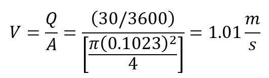
Step 2: Reynolds number

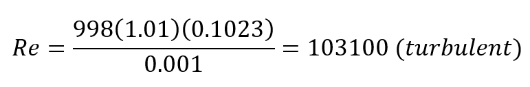
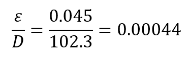
Step 3: Relative roughness

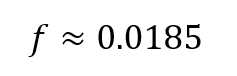
Step 4: Friction factor (Colebrook-White, solved iteratively)

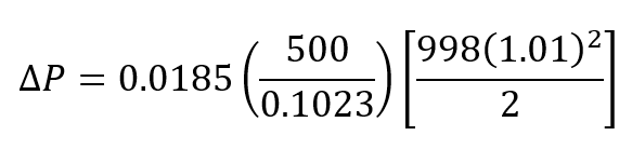
Step 5: Pressure drop (Darcy-Weisbach)

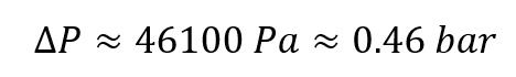
FluidFlow performs this calculation for every pipe segment in the network simultaneously, including the fitting losses, elevation changes, and equipment pressure drops that a hand calculation would handle separately.

---

Frequently Asked Questions

What is the difference between the Darcy friction factor and the Fanning friction factor?

The Darcy friction factor is four times the Fanning friction factor: f_Darcy = 4 × f_Fanning. FluidFlow uses the Darcy convention. When reading data from other sources, check which convention is used. Using the wrong one gives a pressure drop error of 4x.

Why does FluidFlow use Colebrook-White instead of the Moody chart?

The Moody chart is a graphical representation of the Colebrook-White equation. FluidFlow solves Colebrook-White numerically, which is more precise than reading a chart and eliminates interpolation error. The results are the same; the method of obtaining them is more accurate.

When should I use Hazen-Williams instead of Darcy-Weisbach?

Hazen-Williams is simpler (no friction factor iteration) but only valid for water near 15°C in turbulent flow. If you are sizing a water distribution network and your organization uses Hazen-Williams C-factors, FluidFlow supports it. For any other fluid, temperature, or flow regime, use Darcy-Weisbach.

How does pipe ageing affect pressure drop calculations?

Pipe roughness increases over time due to corrosion, scaling, and biological growth. FluidFlow supports pipe scaling factors that increase the effective roughness to represent current pipe condition rather than as-new values. This directly increases the friction factor and pressure drop.

Can I use Darcy-Weisbach for gas flow in FluidFlow?

Darcy-Weisbach can be applied to gas flow under certain assumptions and limitations as described in industry references such as Crane TP-410. Gas behavior is significantly more complex than liquid flow — density, viscosity, and other fluid properties change with both pressure and temperature along the pipe, and these changes must be accounted for to obtain accurate results. Simplified hand-calculation approaches and other hydraulic simulators often rely on assumptions such as isothermal or adiabatic flow, which may not reflect actual operating conditions. FluidFlow addresses these complexities and limitations directly in its gas flow calculations.